Hoàng Phi's Portfolio

What is RFM and K-Mean in Customer Segmentation?

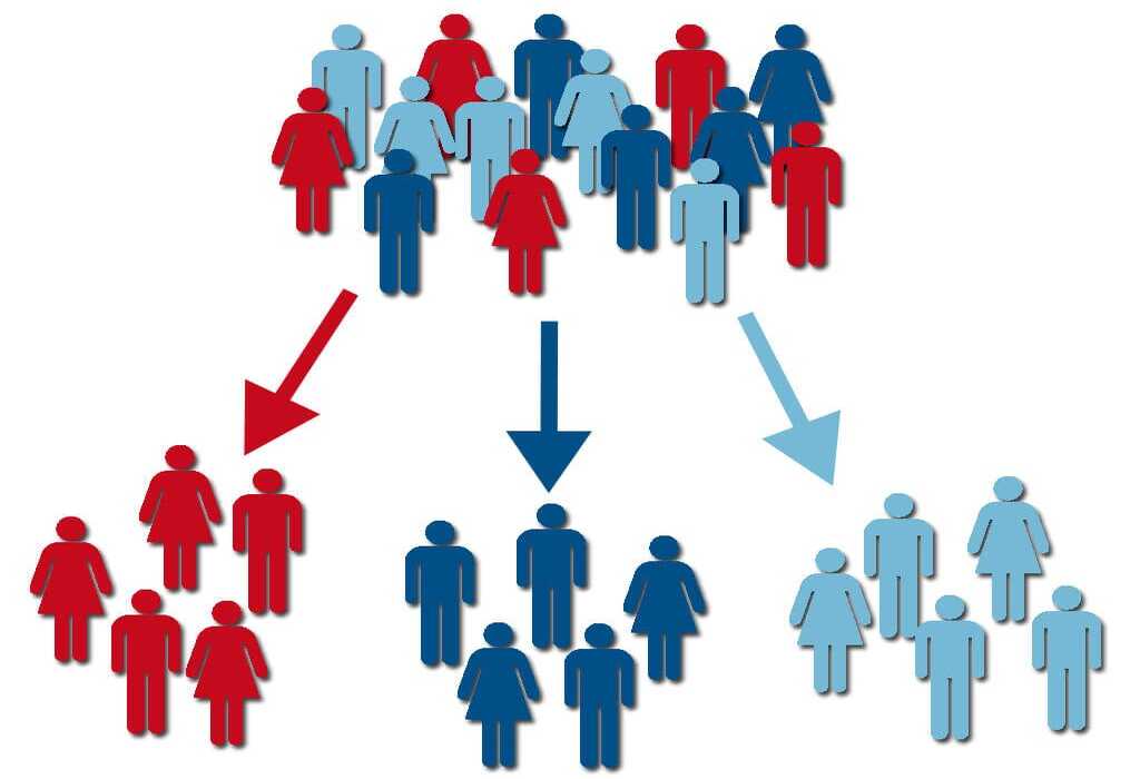
RFM stands for Recency, Frequency, and Monetary Value, and it is a technique used in marketing and customer segmentation to analyze and categorize customers based on their transaction behavior. Each of the three components has a specific meaning:

Recency (R): How recently did the customer make a purchase?

Frequency (F): How often does the customer make purchases within a specific timeframe?

Monetary (M): How much money has the customer spent within a specific timeframe?

K-Means is a clustering algorithm used for partitioning a dataset into a specified number of clusters based on the similarity of data points. When using K-Means with RFM analysis, you are essentially using the three RFM components as features to group similar customers into clusters. The algorithm aims to minimize the variance within each cluster and maximize the variance between clusters.

RFM Customer Segmentation helps businesses better understand their customers, target specific segments with tailored marketing efforts, enhance customer loyalty, and increase profitability through optimized marketing strategies.

The Data Sources

Website Online Retail II

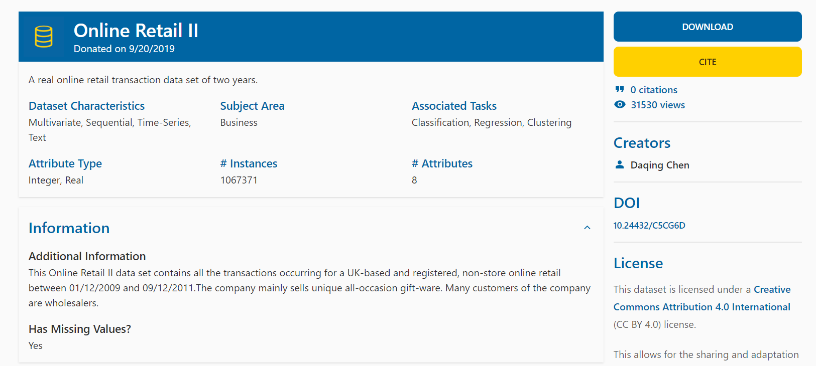
Download dataset in website: Here

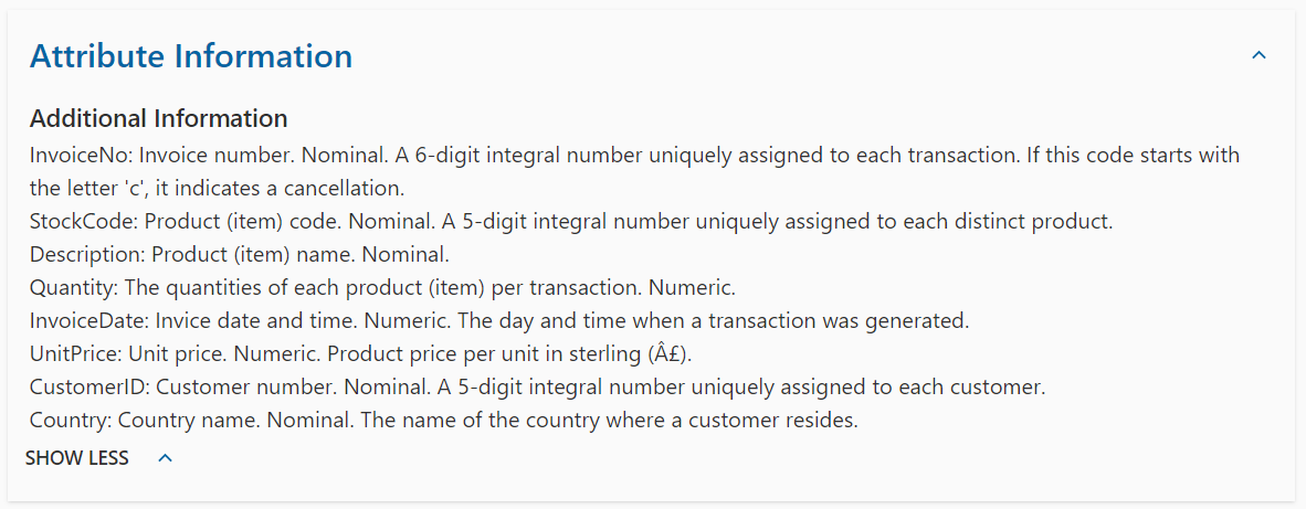
The Dataset Description

Or download dataset in my repository: Here

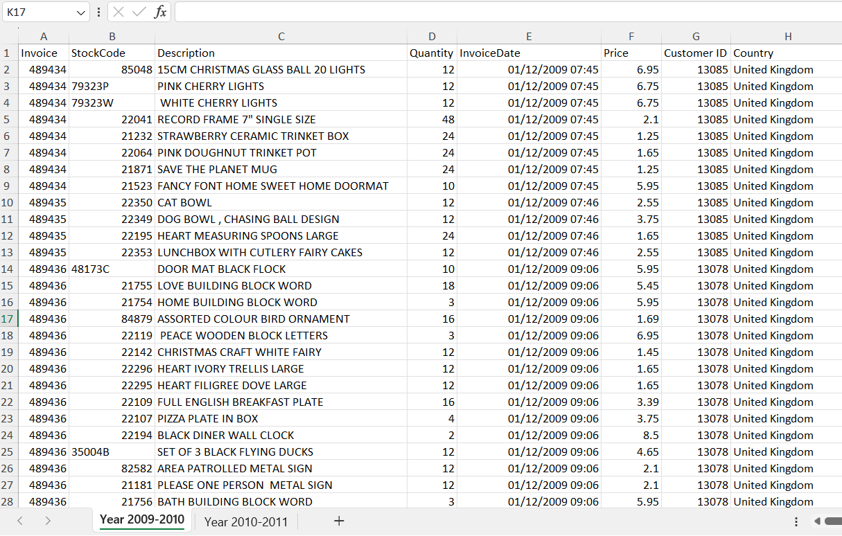
In this project, I only use sheet "Year 2009-2010" for RFM Analysis

Data Cleaning with Python in Google Colab

Import neccessary libraries and read file:

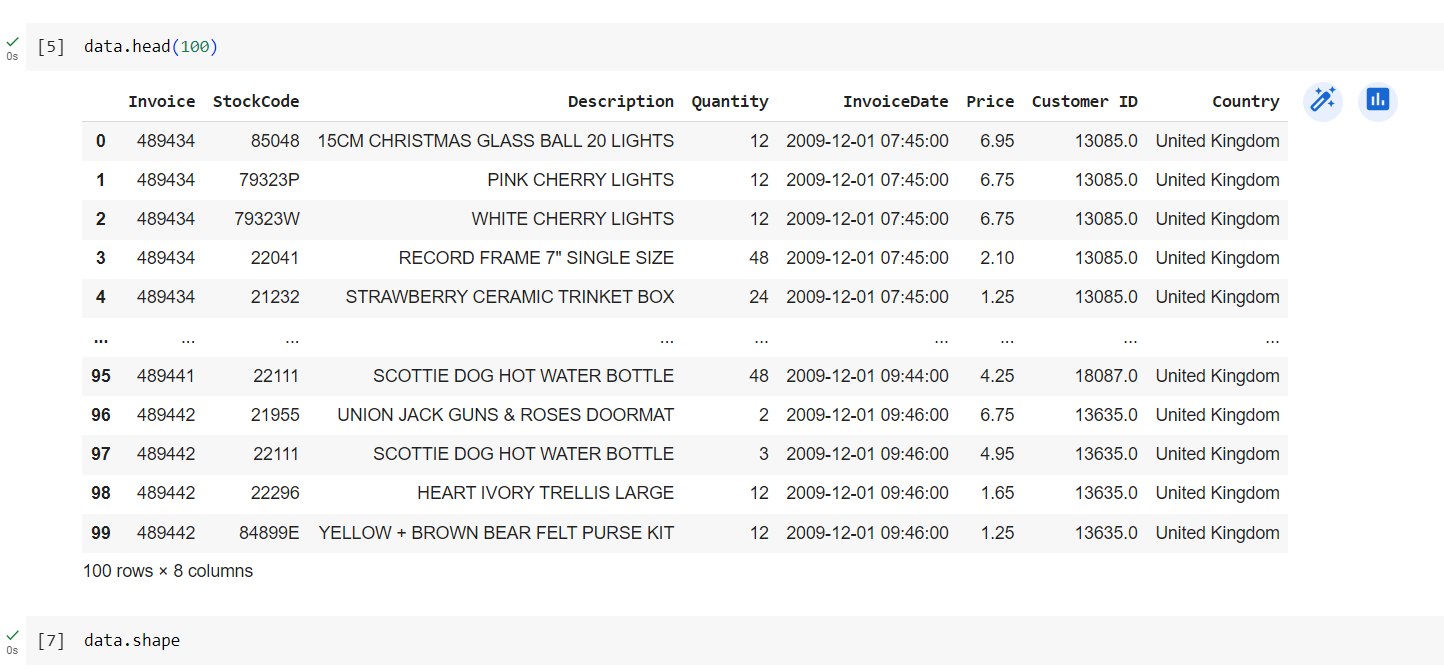
Data overview:

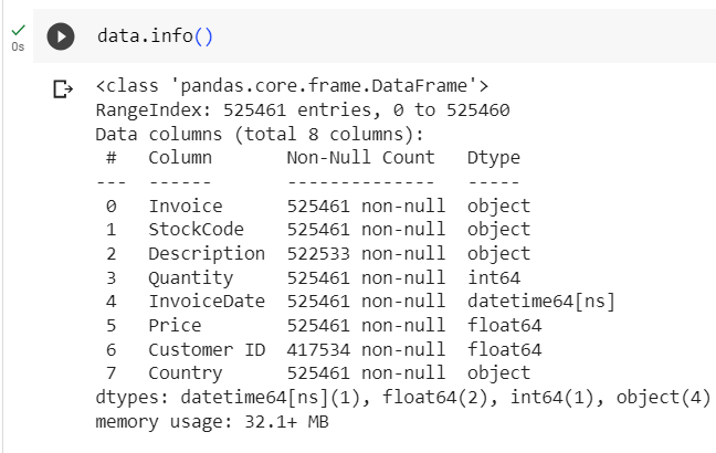
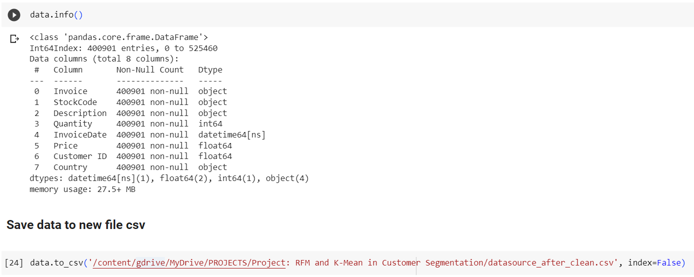
data.info()

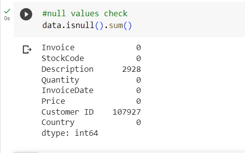
data.isnull().sum()

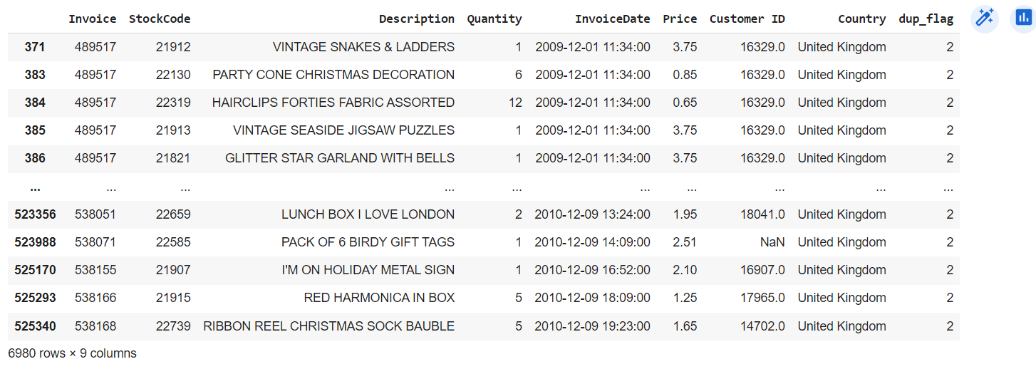
Check duplicated Value
(by this Script)

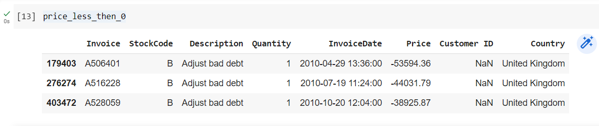
#duplicated values check data = data data['dup_flag'] = data.groupby(['Invoice', 'StockCode', 'Quantity'])['InvoiceDate'].rank(method='first').astype(int) duplicates = data[data['dup_flag'] > 1] duplicates

Price less than 0

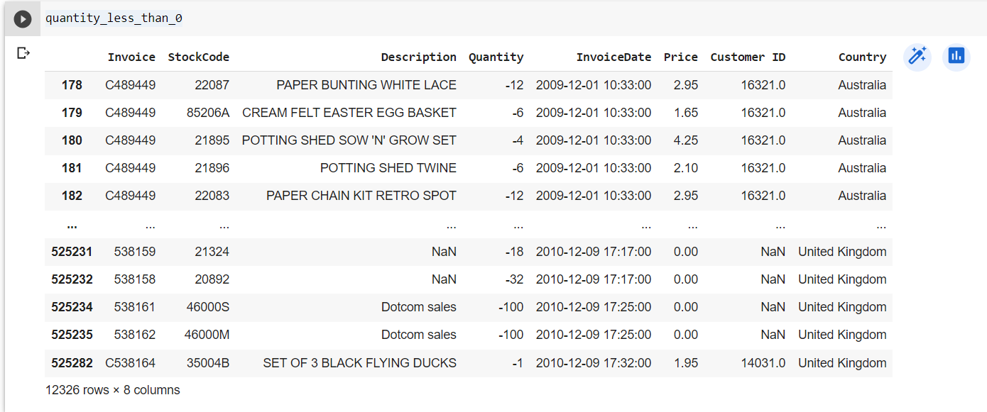
Quantity less than 0

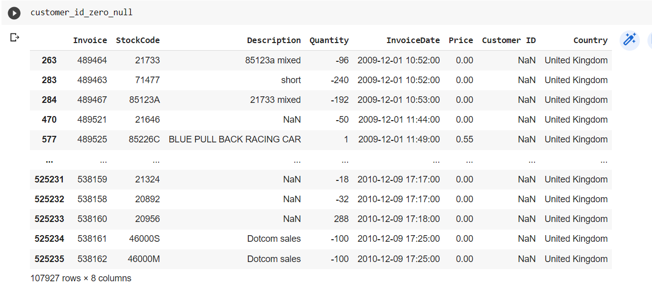
Customer Null and 0

My Exploration

Total Records: 525461 records.

Total Columns: 8 columns.

All columns with correct data type.

There are 2 columns with null values: Description with 2928 and CustomerID with 107927 null values.

There are 12326 records with Quantity less than 0.

There are 3 records with Price less than 0.

There are 107927 records with CustomerId equal 0 and Null values.

There are 6980 records duplicated.

The Scripts of Cleaning

Delete records with Quantity less than 0, UnitPrice less than 0, Customer ID equal to 0, and Customer ID with Null values.

Delete duplicated records.

Each StockCode will correspond to each individual Description. The null Description field may be due to a lack of input by the employee, so the Description can be filled in by checking the StockCode against the previous product.

Here is my code for cleaning in Python:

# Delete records with Quantity < 0 data = data[data['Quantity'] > 0] # Delete records with Price < 0 data = data[data['Price'] > 0] # Delete records with Customer ID = 0 or Customer ID is Null data = data[(data['Customer ID'] != 0) & (data['Customer ID'].notnull())] # Delete duplicated values data['dup_flag'] = data.groupby(['Invoice', 'StockCode', 'Quantity'])['InvoiceDate'].rank(method='first').astype(int) data = data[data['dup_flag'] == 1] data = data.drop(columns=['dup_flag']) # Create a dictionary that maps each StockCode to its corresponding Description stockcode_to_description = data.dropna(subset=['Description']).drop_duplicates('StockCode').set_index('StockCode')['Description'].to_dict() # Filling the missing values in Description # Define a function to fill missing Description based on StockCode def fill_missing_description(row): if pd.isnull(row['Description']): return stockcode_to_description.get(row['StockCode'], None) else: return row['Description'] # Apply the function to the 'Description' column data['Description'] = data.apply(fill_missing_description, axis=1)

Data After Clean (with 400901 Records)
(Save it to new files)

Download the Data After Cleaning: Here

Python Script - Calculate RFM Value

# Calculate RFM # R - Recency Value: current_date = max(data['InvoiceDate']) + dt.timedelta(days=1) # F - Frequency and M - Monetary Value: data['TotalPrice'] = data['Quantity']*data['Price'] rfm_data = data.groupby('Customer ID').agg({ 'InvoiceDate': lambda x: (current_date- x.max()).days, 'Invoice': 'nunique', 'TotalPrice': 'sum' }).reset_index() # Change name rfm_data.columns = ['CustomerID', 'Recency', 'Frequency', 'Monetary'] # Result print(rfm_data)

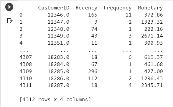
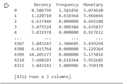
RFM Value Table
(for 4312 CustomerID)

RFM Value Table

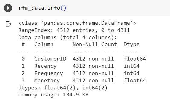
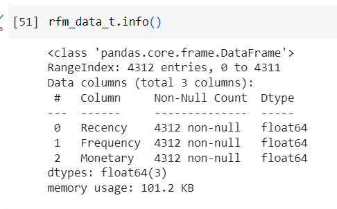
rfm_data.info()

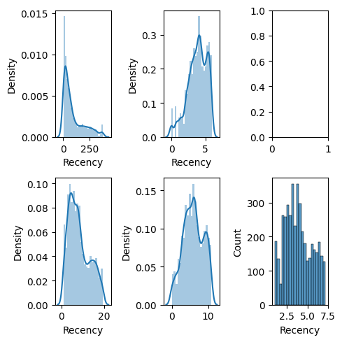
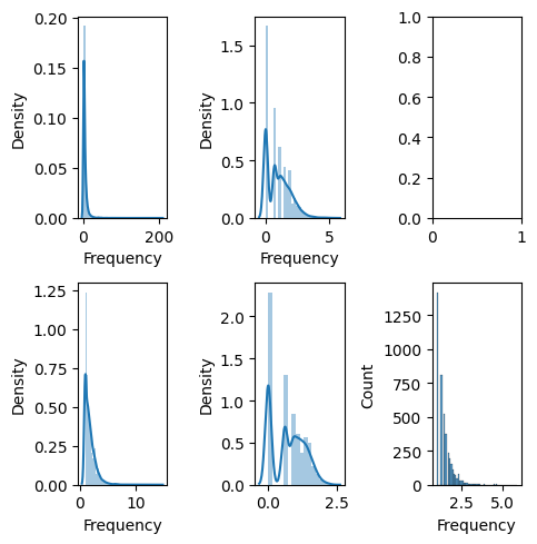
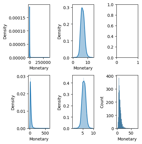
Transformation and Standardization

Display the distribution to check

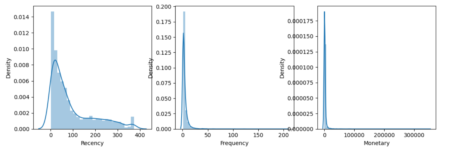
fig, ax = plt.subplots(1, 3, figsize=(15,4)) # Recency distribution sns.distplot(rfm_data['Recency'], ax = ax[0]) # Frequency distribution sns.distplot(rfm_data['Frequency'], ax = ax[1]) # Monetary distribution sns.distplot(rfm_data['Monetary'], ax = ax[2]) plt.show()

We have some problems:

Recency distribution is right-skewed.

Frequency distribution is right-skewed and leptokurtic.

Monetary distribution is right-skewed and leptokurtic.

All three fields do not follow a normal distribution of data.
It is neccessary to transformation data before using K-mean.

Some method for transformation data:

log transformation.

square root transformation.

box-cox transformation.

cube root transformation.

analyze_skewness function:

def analyze_skewness(x): fig, ax = plt.subplots(2,3, figsize=(5,5)) sns.distplot(rfm_data[x], ax=ax[0,0]) sns.distplot(np.log(rfm_data[x]), ax=ax[0,1]) sns.distplot(np.sqrt(rfm_data[x]), ax=ax[1,0]) sns.distplot(stats.boxcox(rfm_data[x])[0], ax=ax[1,2]) sns.histplot(np.cbrt(rfm_data[x]), ax=ax[1, 1]) plt.tight_layout() plt.show() #Print result print("Original Skewness:", rfm_data[x].skew().round(2)) print("Log-transformed Skewness:", np.log(rfm_data[x]).skew().round(2)) print("Square Root-transformed Skewness:", np.sqrt(rfm_data[x]).skew().round(2)) print("Box-Cox transformed Skewness:", pd.Series(stats.boxcox(rfm_data[x])[0]).skew().round(2)) print("Cube Root-transformed Skewness:", pd.Series(np.cbrt(rfm_data[x])).skew().round(2))

analyze_skewness ('Recency')

analyze_skewness ('Frequency')

analyze_skewness ('Monetary')

Original Skewness: 1.28.
Log transformed Skewness: -0.61.
Square Root transformed Skewness: 0.59.
Box-Cox transformed Skewness: -0.07.
Cube root transformed Skewness: 0.27.

Original Skewness: 10.55.
Log transformed Skewness: 0.74.
Square Root transformed Skewness: 3.12.
Box-Cox transformed Skewness: 0.13.
Cube root transformed Skewness: 1.96.

Original Skewness: 24.0.
Log transformed Skewness: 0.25.
Square Root transformed Skewness: 5.8.
Box-Cox transformed Skewness: -0.01.
Cube root transformed Skewness: 2.77.

All data fields are well-suited for Box-Cox transformation as the Box-Cox values are closest to zero.

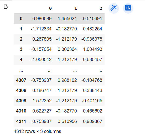
Feature Transformation

rfm_data_t=pd.DataFrame() # Tranform Recency to box-cox transformation rfm_data_t['Recency']=stats.boxcox(rfm_data['Recency'])[0] # Tranform Frequency to box-cox transformation rfm_data_t['Frequency']=stats.boxcox(rfm_data['Frequency'])[0] # Tranform Monetary to box-cox transformation rfm_data_t['Monetary']=stats.boxcox(rfm_data['Monetary'])[0] print(rfm_data_t)

Scaler Data

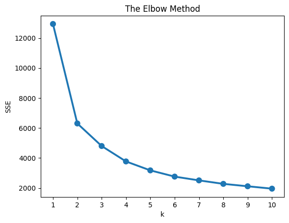
#Scale data from sklearn.preprocessing import StandardScaler scaler = StandardScaler() scaler.fit(rfm_data_t) rfm_data_t_scaler = scaler.transform(rfm_data_t) pd.DataFrame(rfm_data_t_scaler)

Using K-mean to Clustering

Using Elbow to identify the number of cluster

# Use Elbow Method from sklearn.cluster import KMeans sse = {} for k in range(1, 11): kmeans = KMeans(n_clusters=k, random_state=42) kmeans.fit(rfm_data_t_scaler) sse[k] = kmeans.inertia_ # Visualization plt.title('The Elbow Method') plt.xlabel('k') plt.ylabel('SSE') sns.pointplot(x=list(sse.keys()), y=list(sse.values())) plt.show()

Using Silhouette Score to identify the number of cluster

# Using Silhouette Method silhouette_scores = [] possible_k_values = range(2, 11) # k from 2 to 10 for k in possible_k_values: kmeans = KMeans(n_clusters=k, random_state=42) kmeans.fit(rfm_data_t_scaler) labels = kmeans.labels_ silhouette_scores.append(silhouette_score(rfm_data_t_scaler, labels)) # Visualize Silhouette Score for each k value plt.figure(figsize=(10, 6)) plt.plot(possible_k_values, silhouette_scores, marker='o') plt.title('Silhouette Score for Different k') plt.xlabel('Number of Clusters (k)') plt.ylabel('Silhouette Score') plt.xticks(possible_k_values) plt.grid(True) plt.show()

from yellowbrick.cluster import SilhouetteVisualizer # Visualize fig, ax = plt.subplots(2, 2, figsize=(15, 9)) for idx, k in enumerate([2, 3, 4, 5]): km = KMeans(n_clusters=k, init='k-means++', n_init=10, max_iter=100, random_state=42) q, mod = divmod(idx, 2) visualizer = SilhouetteVisualizer(km, colors='yellowbrick', ax=ax[q][mod]) visualizer.fit(rfm_data_t_scaler) ax[q][mod].text(0.5, -0.1, f'Silhouette Score: {np.mean(visualizer.silhouette_score_):.2f}', size=12, ha='center', transform=ax[q][mod].transAxes) plt.tight_layout() plt.show()

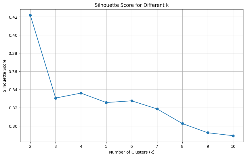
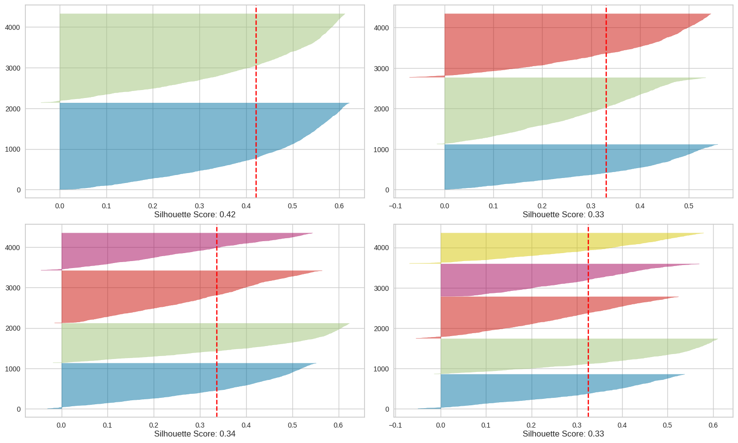
As the graph visualized above is:

In both two method, we won't choose k =2 because it doesn't has the good cluster.

In the Elbow method, we will choose k = 4 because this score represents a relatively large reduction in SSE compared to the previous k.

In the Silhouette method, we will choose k = 4 because with k = 4 having highest Silhouette Score and the number of good clusters.

So I choose k = 4 for clustering

Clustering

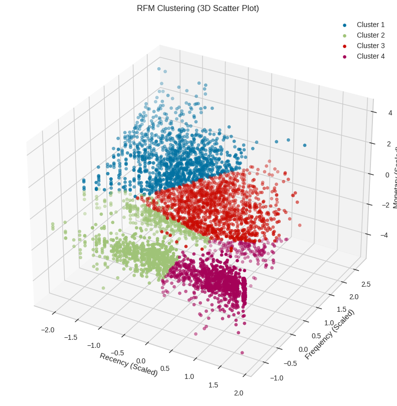
from mpl_toolkits.mplot3d import Axes3D #Choose k = 4 and fit it with data k = 4 kmeans = KMeans(n_clusters=k, init='k-means++', n_init=10, max_iter=100, random_state=42) clusters = kmeans.fit_predict(rfm_data_t_scaler) rfm_data_t_scaler['Cluster'] = clusters rfm_data['Cluster'] = clusters # Visualize with 3D graph by Recency, Frequency and Monetary fig = plt.figure(figsize=(13, 10)) ax = fig.add_subplot(111, projection='3d') for i in range(k): cluster_data = rfm_data_t_scaler[rfm_data_t_scaler['Cluster'] == i] ax.scatter(cluster_data['Recency'], cluster_data['Frequency'], cluster_data['Monetary'], label=f'Cluster {i+1}') ax.set_xlabel('Recency (Scaled)') ax.set_ylabel('Frequency (Scaled)') ax.set_zlabel('Monetary (Scaled)') ax.set_title('RFM Clustering (3D Scatter Plot)') ax.legend() plt.show()

This is data After clustering. We can see that the data is clustered.

Group data by cluster and Analysis

rfm_data.groupby('Cluster').agg( { 'Recency':'mean', 'Frequency':'mean', 'Monetary':'mean' } ).round(2)

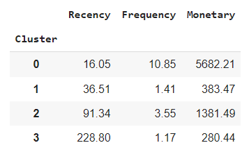
Cluster 0 - "Loyal High-Spending Customers":

Metric:

Recency: 16.05 (Recent)

Frequency: 10.85 (Frequent)

Monetary: 5682.21 (High spending)

This segment comprises customers who have made recent, frequent purchases and have a high spending level. They might be loyal and significant customers for your business.
Marketing strategies for this group could include:

Special offers: Provide exclusive discounts, special offers, or gifts for their next purchase to honor their loyalty.

Membership program: Encourage them to join a loyalty program to receive more benefits from their shopping.

Cluster 1 - "Infrequent Low-Spending Customers":

Metric:

Recency: 36.51 (Quite a while)

Frequency: 1.41 (Infrequent)

Monetary: 383.47 (Low spending)

This segment consists of customers who make infrequent purchases with low spending. They could be potential customers that need to be motivated to increase their purchases and spending.
Marketing strategies for this group could include:

Re-engagement campaigns: Send emails or push notifications with appealing offers to encourage them to return for shopping.

Bundle promotions: Offer additional products or services with their orders to enhance the value of their purchases.

Cluster 2 - "Occasional Medium-Spending Customers":

Metric:

Recency: 91.34 (Quite a while)

Frequency: 3.55 (Infrequent)

Monetary: 1381.49 (Moderate spending)

This segment includes customers who shop occasionally with moderate spending. They have the potential to increase their purchases if motivated appropriately.
Marketing strategies for this group could include:

Stimulus campaigns: Use email marketing or advertisements to introduce new and attractive products.

Loyalty points program: Encourage them to shop more frequently by offering loyalty points that can be redeemed for rewards.

Cluster 3 - "Rare Low-Spending Inactive Customers":

Metric:

Recency: 228.80 (Quite a while)

Frequency: 1.17 (Infrequent)

Monetary: 280.44 (Moderate spending)

This segment contains customers who rarely shop, haven't been active recently, and have low spending. They might be challenging to re-engage.
Marketing strategies for this group could include:

Recovery campaigns: Use email marketing or advertisements to introduce new and attractive products.

Feedback surveys: Gather their opinions about products or services to improve their shopping experience and attract them back.

View my full project: Here

Skill:

Previous Post Next Post

RFM WITH K-MEAN IN CUSTOMER SEGMENTATION

Using Python (Cleaning, Transformation, Standardization, Visualization) and K-Mean (Clustering)