What is Stock Price Prediction?
Stock Price Prediction is one of the most popular problems in the series of related problems regarding Time Series data. There, we will use the indicators recorded in the past of a stock and predict its price in the future, so that appropriate investment decisions can be made.
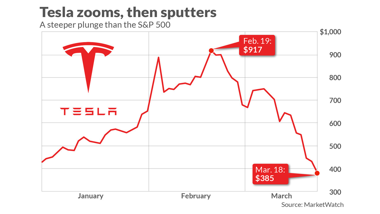
For stock investors who rely on the method of technical analysis (Technical Analysis), they often rely on the adjusted closing price of the stock to make decisions to buy/sell stocks. Therefore, in this project, we will build a model that predicts the adjusted closing price of Tesla company stock based on the indices recorded on stock trading days in the period from 06 /29/2010 to 03/17/2017.
Understand the Input and Output
Input / Output of this project is:
Input: Indexes of stocks in the previous 30 trading days.
Output: Adjusted Closing Price of the current day.
The Data Sources
The time - series data
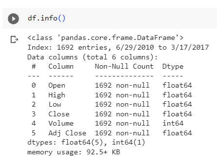
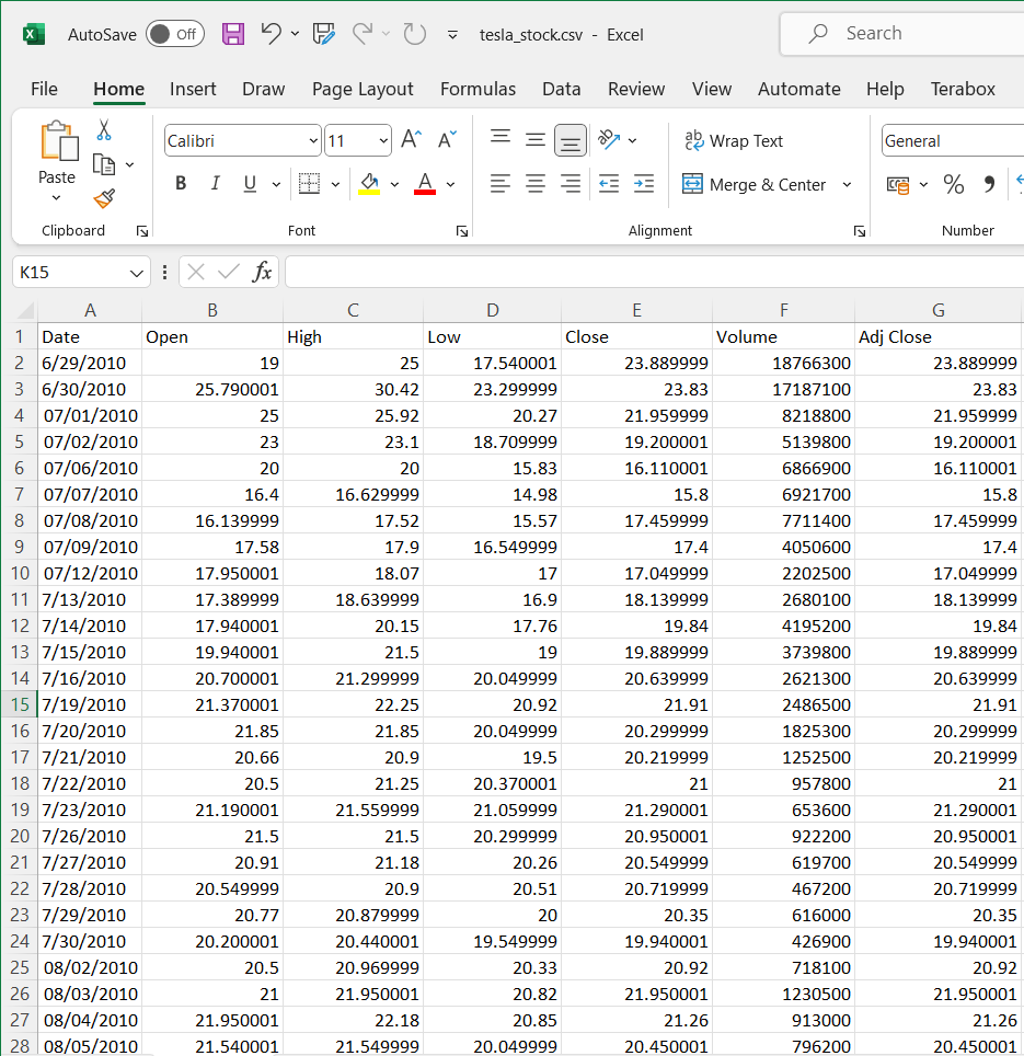
File data source with columns: Date, Open, High, Low, Close, Volume, Adj Close.
Download dataset in my repository: Here
The Pipe Line
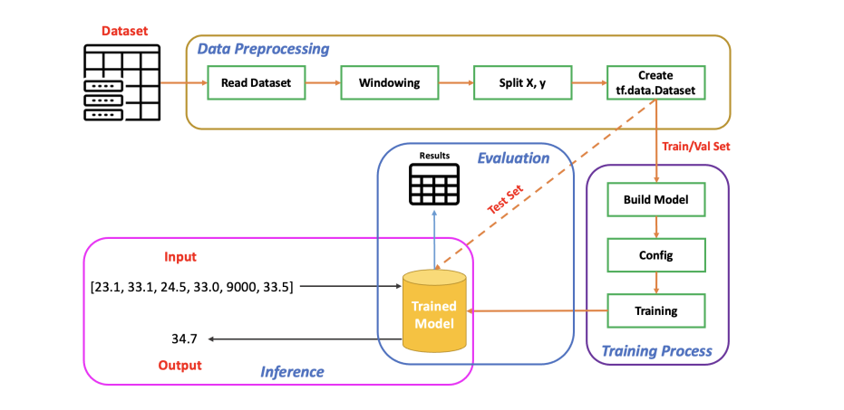
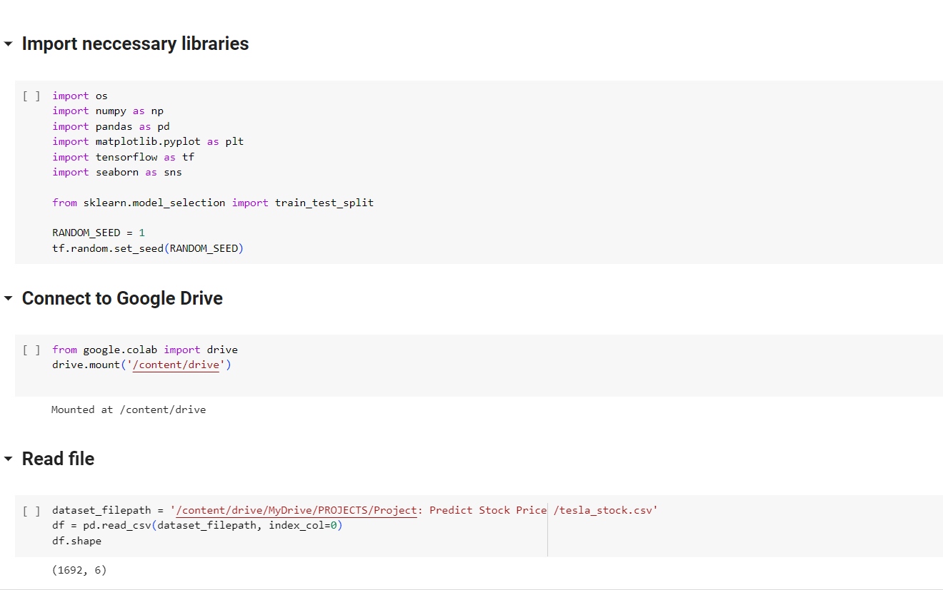
Import necessary libraries and Read File
EDA Dataset
df.head()
.PNG)
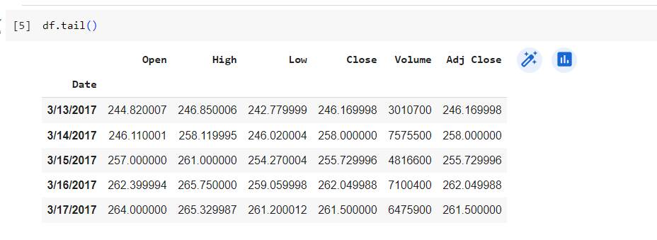
df.tail()
- Date: Transaction date.
- Open: Opening price.
- High: The highest price of the day.
- Low: Lowest price of the day.
- Close: The closing price.
- Volume: Trading volume.
- Adj Close: Corrective closing price.
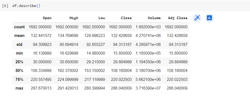
df.describe()
Visualization
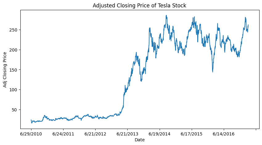
# Visualization of Adjusted Closing Price of Tesla Stock
plt.figure(figsize=(10, 5))
df['Adj Close'].plot()
plt.title('Adjusted Closing Price of Tesla Stock')
plt.xlabel('Date')
plt.ylabel('Adj Closing Price')
plt.show()
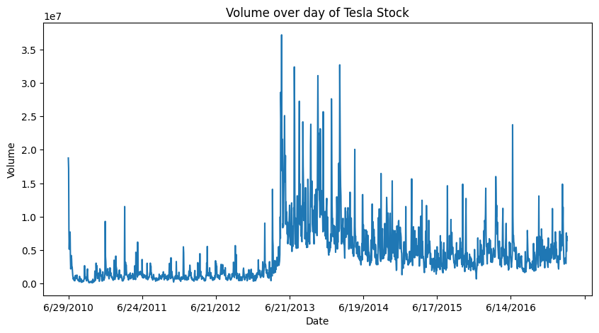
# Visualization of Volume overday of Tesla Stock
plt.figure(figsize=(10, 5))
df['Volume'].plot()
plt.title('Volume over day of Tesla Stock')
plt.xlabel('Date')
plt.ylabel('Volume')
plt.show()
Data Preparation
Use Slicing Windowing Method
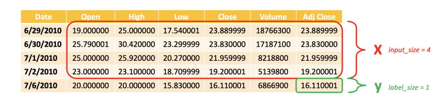
# Declare the Windowing function (used to create X, y pairs for time series data)
def slicing_window(df, df_start_idx, df_end_idx, input_size, label_size, offset, label_name):
features = [] # Declare a list to store X
labels = [] # Declare a list to store y
# If df_end_idx equals the last index of the data frame, need to move down by a window size
if df_end_idx == None:
df_end_idx = len(df) - label_size - offset
df_start_idx = df_start_idx + input_size + offset
# Iterate through each data sample
for idx in range(df_start_idx, df_end_idx):
feature_start_idx = idx - input_size - offset
feature_end_idx = feature_start_idx + input_size
label_start_idx = idx - 1
label_end_idx = label_start_idx + label_size
feature = df[feature_start_idx:feature_end_idx] # Get X
label = df[label_name][label_start_idx:label_end_idx] # Get y
features.append(feature)
labels.append(label)
# Convert lists to np.ndarrays
features = np.array(features)
labels = np.array(labels)
return features, labels
Split to Train / Val / Test
dataset_length = len(df) # Number of data samples in the DataFrame
TRAIN_SIZE = 0.7 # Training set ratio
VAL_SIZE = 0.2 # Validation set ratio
# Convert ratios to indices
TRAIN_END_IDX = int(TRAIN_SIZE * dataset_length)
VAL_END_IDX = int(VAL_SIZE * dataset_length) + TRAIN_END_IDX
Make a function call
INPUT_SIZE = 30
LABEL_SIZE = 1
OFFSET = 1
BATCH_SIZE = 64
TARGET_NAME = 'Adj Close'
# Initialize X, y for the training set
X_train, y_train = slicing_window(df,
df_start_idx=0,
df_end_idx=TRAIN_END_IDX,
input_size=INPUT_SIZE,
label_size=LABEL_SIZE,
offset=OFFSET,
label_name=TARGET_NAME)
# Initialize X, y for the validation set
X_val, y_val = slicing_window(df,
df_start_idx=TRAIN_END_IDX,
df_end_idx=VAL_END_IDX,
input_size=INPUT_SIZE,
label_size=LABEL_SIZE,
offset=OFFSET,
label_name=TARGET_NAME)
# Initialize X, y for the test set
X_test, y_test = slicing_window(df,
df_start_idx=VAL_END_IDX,
df_end_idx=None,
input_size=INPUT_SIZE,
label_size=LABEL_SIZE,
offset=OFFSET,
label_name=TARGET_NAME)
Create tf.data.Dataset
for the convenience of training in Tensorflow
# Initilize tf.data.Dataset
train_ds = tf.data.Dataset.from_tensor_slices((X_train, y_train)).batch(BATCH_SIZE)
val_ds = tf.data.Dataset.from_tensor_slices((X_val, y_val)).batch(BATCH_SIZE)
test_ds = tf.data.Dataset.from_tensor_slices((X_test, y_test)).batch(BATCH_SIZE)
# Configuring and Preparing Data
AUTOTUNE = tf.data.AUTOTUNE
train_ds = train_ds.cache().prefetch(buffer_size=AUTOTUNE)
val_ds = val_ds.cache().prefetch(buffer_size=AUTOTUNE)
Build Model
# Normalization layer
normalize_layer = tf.keras.layers.Normalization()
normalize_layer.adapt(np.vstack((X_train, X_val, X_test)))
# Build model
def build_model(input_shape, output_size):
input_layer = tf.keras.Input(shape=input_shape, name='input_layer')
x = normalize_layer(input_layer)
for n_unit in [128, 64]:
rnn_x = tf.keras.layers.SimpleRNN(n_unit,
return_sequences=True,
kernel_initializer=tf.initializers.GlorotUniform(seed=RANDOM_SEED)
)(x)
lstm_x = tf.keras.layers.LSTM(n_unit,
return_sequences=True,
kernel_initializer=tf.initializers.GlorotUniform(seed=RANDOM_SEED)
)(x)
x = tf.concat([rnn_x, lstm_x], axis=-1)
rnn_x = tf.keras.layers.SimpleRNN(n_unit,
return_sequences=False,
kernel_initializer=tf.initializers.GlorotUniform(seed=RANDOM_SEED)
)(x)
lstm_x = tf.keras.layers.LSTM(n_unit,
return_sequences=False,
kernel_initializer=tf.initializers.GlorotUniform(seed=RANDOM_SEED)
)(x)
x = tf.concat([rnn_x, lstm_x], axis=-1)
x = tf.keras.layers.Dense(32,
activation='relu',
kernel_initializer=tf.initializers.GlorotUniform(seed=RANDOM_SEED),
name='fc_layer_1'
)(x)
output_layer = tf.keras.layers.Dense(output_size,
kernel_initializer=tf.initializers.GlorotUniform(seed=RANDOM_SEED),
name='output_layer')(x)
model = tf.keras.Model(input_layer, output_layer, name='combined_model')
return model
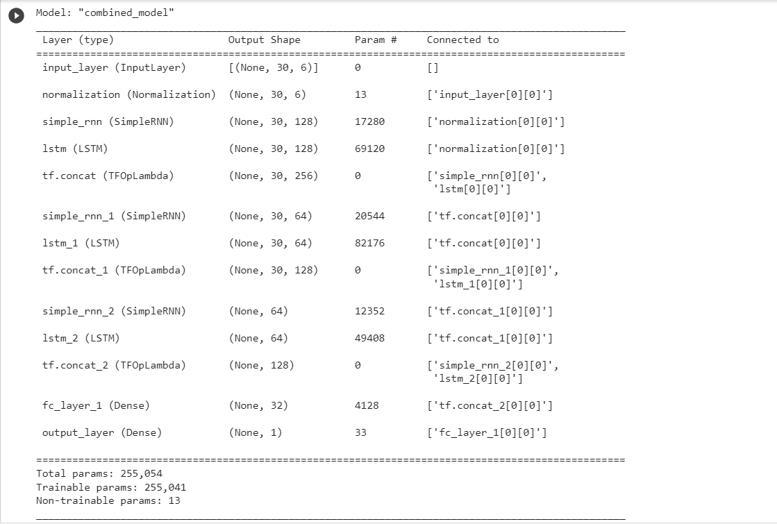
# Summary of model
INPUT_SHAPE = X_train.shape[-2:]
model = build_model(INPUT_SHAPE,
LABEL_SIZE)
model.summary()
Setting other parameters for the model
# hyperparameter values
EPOCHS = 500
LR = 1e-3
# Some optimization for model
model.compile(
optimizer=tf.keras.optimizers.Adam(learning_rate=LR), # Use optimizer Adam
loss=tf.keras.losses.MeanSquaredError(), # Use loss Mean Squared Error Function
)
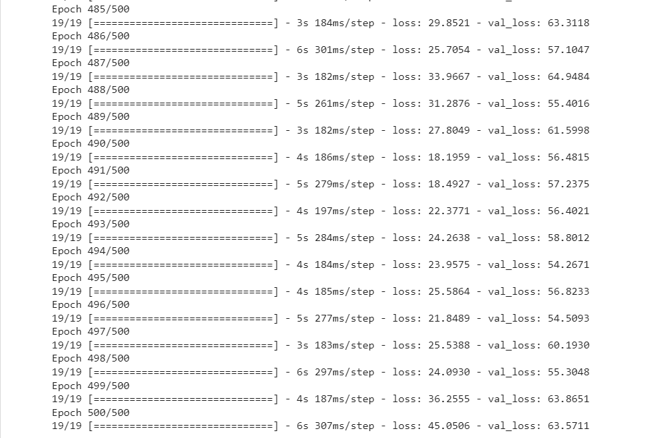
Training Model
history = model.fit(train_ds,
validation_data=val_ds,
epochs=EPOCHS)
Model Evalutation
# Define MAE
def mae(y_true, y_pred):
mae = np.mean(np.abs((y_true - y_pred)))
return mae
# Define MSE
def mse(y_true, y_pred):
mse = np.mean((y_true - y_pred) ** 2)
return mse
# Define RMSE
def rmse(y_true, y_pred):
rmse = np.sqrt(np.mean((y_true-y_pred)**2))
return rmse
# Define MAPE
def mape(y_true, y_pred):
mape = np.mean(np.abs((y_true-y_pred) / y_true)) * 100
return mape
# Print result
y_test_pred = model.predict(X_test, verbose=0)
print(f'RMSE: {rmse(y_test, y_test_pred)}')
print(f'MAPE: {mape(y_test, y_test_pred)}')
print(f'MSE: {mse(y_test, y_test_pred)}')
print(f'MAE: {mae(y_test, y_test_pred)}')
The result is:
- RMSE: 7.08275569019287
- MAPE: 2.698402709155248
- MSE: 50.16542816695947
- MAE: 5.680429943373632
Visualization Result
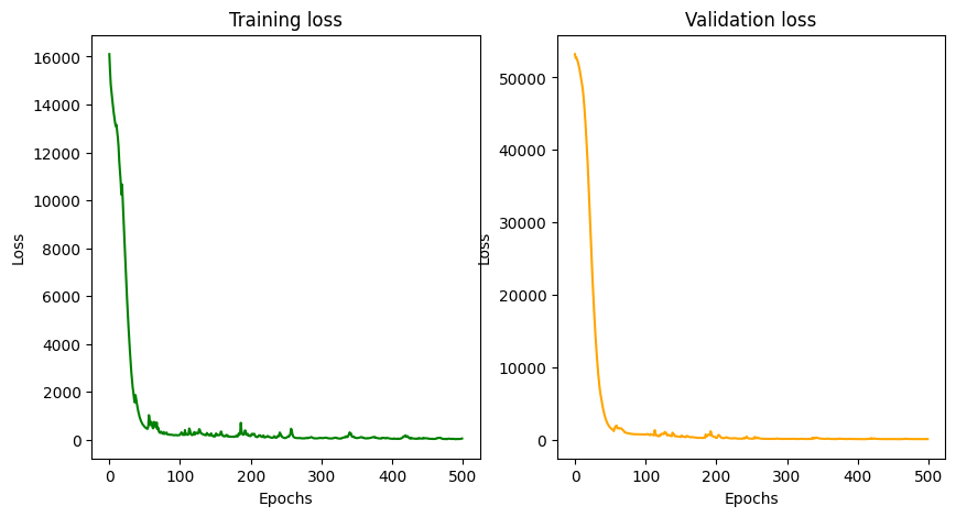
Visualize loss / accuracy results during training
train_loss = history.history['loss'] # Read training loss information
val_loss = history.history['val_loss'] # Read validation loss information
plt.figure(figsize=(10, 5)) # Set the figure size
plt.subplot(1, 2, 1) # Initialize the plot for training loss
plt.xlabel('Epochs') # Display the x-axis label as 'Epochs'
plt.ylabel('Loss') # Display the y-axis label as 'Loss'
plt.title('Training loss') # Display the title of the current plot as 'Training Loss'
plt.plot(train_loss, color='green') # Plot the training loss values over epochs (plotting in green)
plt.subplot(1, 2, 2) # Initialize the plot for validation loss
plt.xlabel('Epochs') # Display the x-axis label as 'Epochs'
plt.ylabel('Loss') # Display the y-axis label as 'Loss'
plt.title('Validation loss') # Display the title of the current plot as 'Validation loss'
plt.plot(val_loss, color='orange') # Plot the validation loss values over epochs (plotting in orange)
plt.show() # Display both small plots
Visualize the predicted value compared to the actual value on the test set
def plot_difference(y, pred):
plt.figure(figsize=(20, 6))
times = range(len(y))
y_to_plot = y.flatten()
pred_to_plot = pred.flatten()
plt.plot(times, y_to_plot, color='steelblue', marker='o', label='True value')
plt.plot(times, pred_to_plot, color='orangered', marker='X', label='Prediction')
plt.title('Adj Closing Price per day')
plt.xlabel('Date')
plt.ylabel('Adj Close Price')
plt.legend()
plt.show()
plot_difference(y_test[:300], model.predict(X_test[:300], verbose=0))
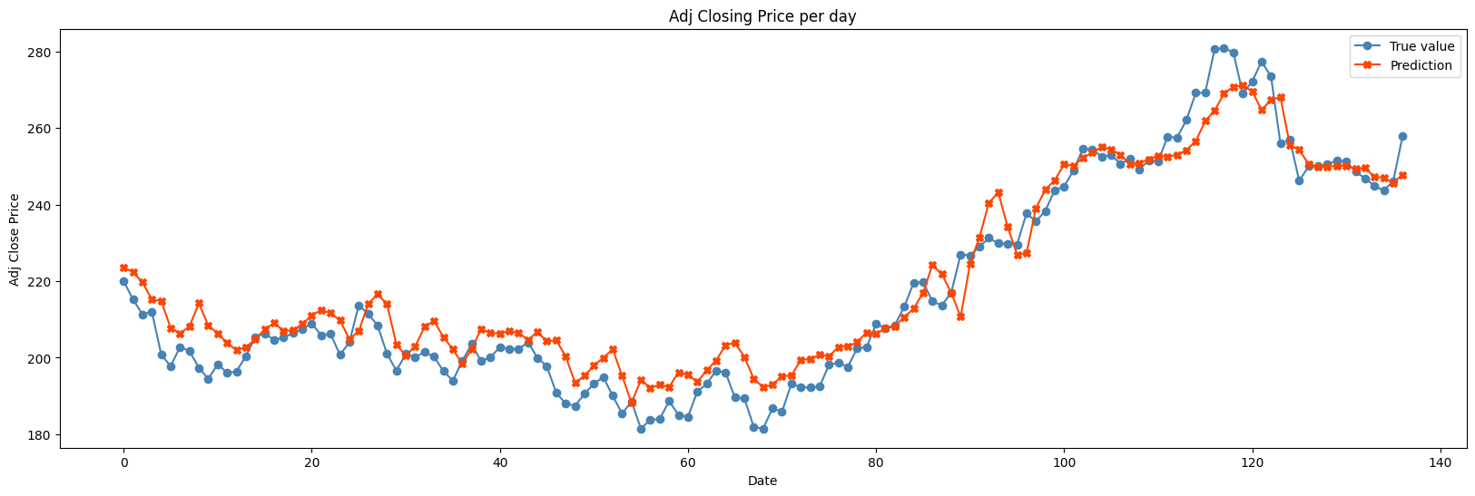
Based on low-value MAE, MSE, RMSE and MAPE metrics, as well as training loss visualization, validation loss, and predicted versus true value visualization on the test set, it is possible concluded that the model performed well in predicting Tesla's stock price!
View my full project: Here